Python and 3PCF Tutorial
This section provides a practical example of how to use 3ptWL-mod from a Python notebook. The example follows a complete workflow:
Generate a linear matter power spectrum using CAMB.
Run
wlcfthrough the Python wrapper.Plot the resulting 3-point correlation function multipoles.
Compare different theoretical models.
The notebook associated with this tutorial can be used as a starting point for interactive runs and parameter exploration. For a shorter workflow that does not require a repository checkout or CAMB, begin with the standalone Google Colab: Four-Model Comparison notebook.
Setting up the working directory
First, import the required Python packages and move to the tests directory
of the repository:
import os
import numpy as np
import matplotlib.pyplot as plt

import camb
from camb import model
from wlcfpy import wlcf

WLCF_TESTS_DIR = os.environ.get("WLCF_TESTS_DIR", "/path/to/3ptWL-mod/tests")
os.chdir(WLCF_TESTS_DIR)

os.makedirs("input", exist_ok=True)
os.makedirs("Output", exist_ok=True)
Generating the linear power spectrum
The linear matter power spectrum can be generated with CAMB. In this example we use a T17-like cosmology at redshift \(z = 0.5078\):
def make_camb_linear_pk(
    output_file="./input/linear_pk_camb_T17_z05078.txt",
    z_pk=0.5078,
    h=0.7,
    Omb=0.046,
    Omc=0.233,
    Omnu=0.0,
    ns=0.97,
    sigma8=0.82,
    w0=-1.0,
    kmin=1e-4,
    kmax=50.0,
    npoints=1000,
):

    os.makedirs(os.path.dirname(output_file), exist_ok=True)

    H0 = 100.0 * h
    ombh2 = Omb * h**2
    omch2 = Omc * h**2

    pars = camb.CAMBparams()

    # For now we assume massless neutrinos, consistent with Omnu = 0.
    pars.set_cosmology(
        H0=H0,
        ombh2=ombh2,
        omch2=omch2,
    )

    pars.InitPower.set_params(
        ns=ns,
        As=2.1e-9
    )

    pars.set_dark_energy(w=w0)

    # Linear power spectrum at the same redshift used by wlcf/zbin
    pars.set_matter_power(
        redshifts=[z_pk],
        kmax=kmax
    )

    pars.NonLinear = model.NonLinear_none

    # First run to compute sigma8 for the trial As
    results = camb.get_results(pars)
    sigma8_current = results.get_sigma8()[0]

    # Rescale As so that CAMB matches the requested sigma8
    As_rescaled = 2.1e-9 * (sigma8 / sigma8_current) ** 2

    pars.InitPower.set_params(
        ns=ns,
        As=As_rescaled
    )

    results = camb.get_results(pars)

    kh, redshifts, pk = results.get_matter_power_spectrum(
        minkh=kmin,
        maxkh=kmax,
        npoints=npoints,
    )

    pk_z = pk[0]

    np.savetxt(
        output_file,
        np.column_stack([kh, pk_z]),
        fmt="%.10e"
    )

    print(f"Saved linear P(k) at z={z_pk} to:")
    print(output_file)
    print(f"sigma8 target  = {sigma8}")
    print(f"sigma8 CAMB    = {results.get_sigma8()[0]:.6f}")
    print(f"As rescaled    = {As_rescaled:.6e}")

    return output_file, kh, pk_z
The resulting file is passed to wlcf through the parameter fnamePS.
Running 3ptWL-mod from Python
The code can be executed directly from Python using the wlcfpy wrapper:
w = wlcf()
w.set(
    numberThreads=8,
    verbose=2,
    verbose_log=1,

    z=0.5078,
    h=0.7,
    sigma8=0.82,
    Omb=0.046,
    Omc=0.233,
    Omnu=0.0,
    ns=0.97,
    w=-1.0,

    fnamePS="./input/linear_pk_camb_T17_z05078.txt",
    Wg=0,
    fWgchi="./input/Wg_Takahashi_z05078.txt",

    rootDir="Output",
    prefix="halo_model_z05078_",

    tree_level=4,
    zbin=0.5078,
    mMax=5,
    chiQuadSteps=300,
    GLpoints=64,
    Nell=128,
    ellmax=10000,
    ellmin=0.001,
    writevectors=0,
    options=""
)

w.Run()
Here tree_level=4 selects the Takahashi/Halo-model branch.
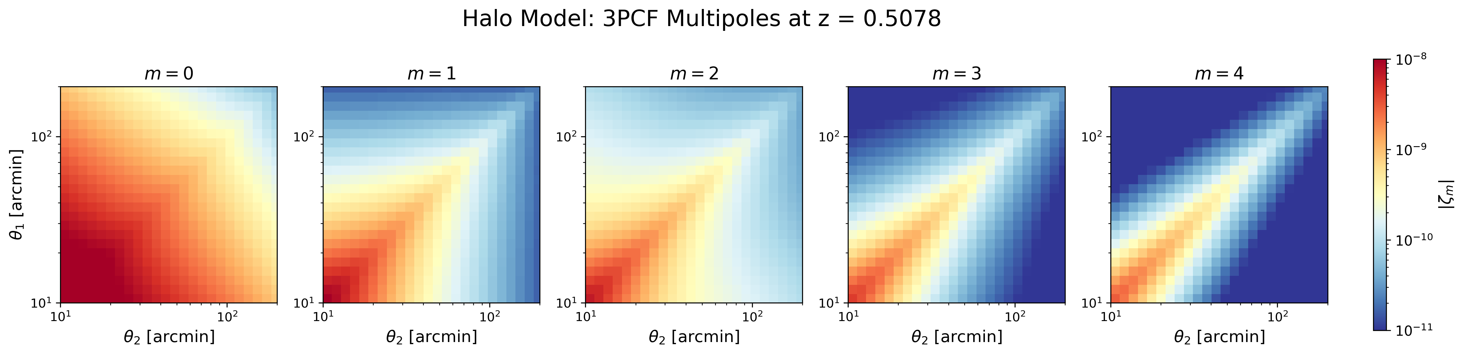
Plotting the 3PCF multipoles
The output files zetam*.txt contain the multipoles
\(\zeta_m(\theta_1,\theta_2)\). These can be visualized as 2D maps:
import numpy as np
import matplotlib.pyplot as plt
from matplotlib.colors import LogNorm

path = "Output"
prefix = "halo_model_z05078_"

theta = np.loadtxt(f"{path}/{prefix}theta_array.txt") * 180 / np.pi * 60
Theta2, Theta1 = np.meshgrid(theta, theta)

fig = plt.figure(figsize=(19, 4))

gs = fig.add_gridspec(
    nrows=1,
    ncols=6,
    width_ratios=[1, 1, 1, 1, 1, 0.06],
    wspace=0.25
)

norm = LogNorm(vmin=1e-11, vmax=1e-8)

for m in range(5):
    ax = fig.add_subplot(gs[0, m])

    zeta = np.abs(np.loadtxt(f"{path}/{prefix}zetam{m}.txt"))

    im = ax.pcolormesh(
        Theta2,
        Theta1,
        zeta,
        shading="auto",
        cmap="RdYlBu_r",
        norm=norm
    )

    ax.set_xscale("log")
    ax.set_yscale("log")
    ax.set_xlim(10, 200)
    ax.set_ylim(10, 200)
    ax.set_aspect("equal", adjustable="box")
    ax.set_title(fr"$m={m}$", fontsize=14)

    if m == 0:
        ax.set_ylabel(r"$\theta_1$ [arcmin]", fontsize=13)

    ax.set_xlabel(r"$\theta_2$ [arcmin]", fontsize=13)

# Colorbar outside the plots
cax = fig.add_subplot(gs[0, -1])
cbar = fig.colorbar(im, cax=cax)
cbar.set_label(r"$|\zeta_m|$", fontsize=13)
cbar.ax.tick_params(labelsize=11)

fig.suptitle(
    "Halo Model: 3PCF Multipoles at z = 0.5078",
    fontsize=18,
    y=1.02
)
plt.savefig("halo_model_3pcf.png", dpi=300, bbox_inches="tight")
plt.show()
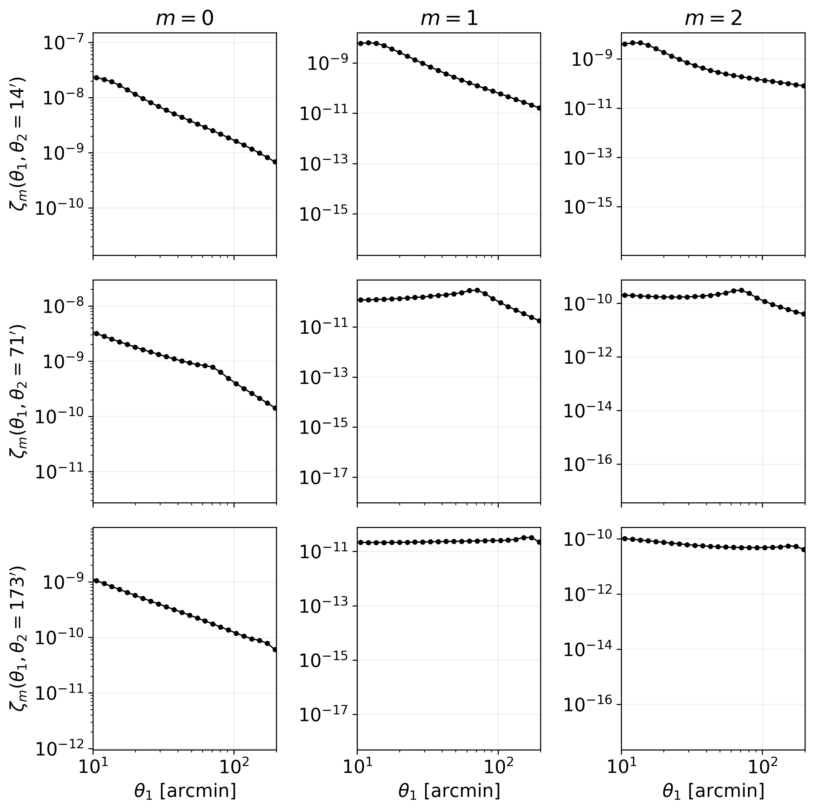
Or we can plot
path = "Output"
prefix = "halo_model_z05078_"

theta = np.loadtxt(f"{path}/{prefix}theta_array.txt") * 180/np.pi * 60

theta2_targets = [13, 72, 169]
m_values = [0, 1, 2]

fig, axes = plt.subplots(
    len(theta2_targets),
    len(m_values),
    figsize=(9, 9),
    sharex=True
)

for i, theta2_fixed in enumerate(theta2_targets):
    idx = np.argmin(np.abs(theta - theta2_fixed))
    theta2_actual = theta[idx]

    for j, m in enumerate(m_values):
        ax = axes[i, j]

        zeta = np.abs(np.loadtxt(f"{path}/{prefix}zetam{m}.txt"))

        # theta2 fixed, theta1 varies
        y = zeta[:, idx]

        ax.plot(theta, y, color="black", marker="o", markersize=3, lw=1)

        ax.set_xscale("log")
        ax.set_yscale("log")

        ax.set_xlim(10, 200)

        if i == 0:
            ax.set_title(fr"$m={m}$")

        if j == 0:
            ax.set_ylabel(
                fr"$\zeta_m(\theta_1,\theta_2={theta2_actual:.0f}')$"
            )

        if i == len(theta2_targets) - 1:
            ax.set_xlabel(r"$\theta_1$ [arcmin]")

        ax.grid(alpha=0.2)

plt.tight_layout()
plt.savefig("halo_model_slice_3pcf.png", dpi=300, bbox_inches="tight")
plt.show()
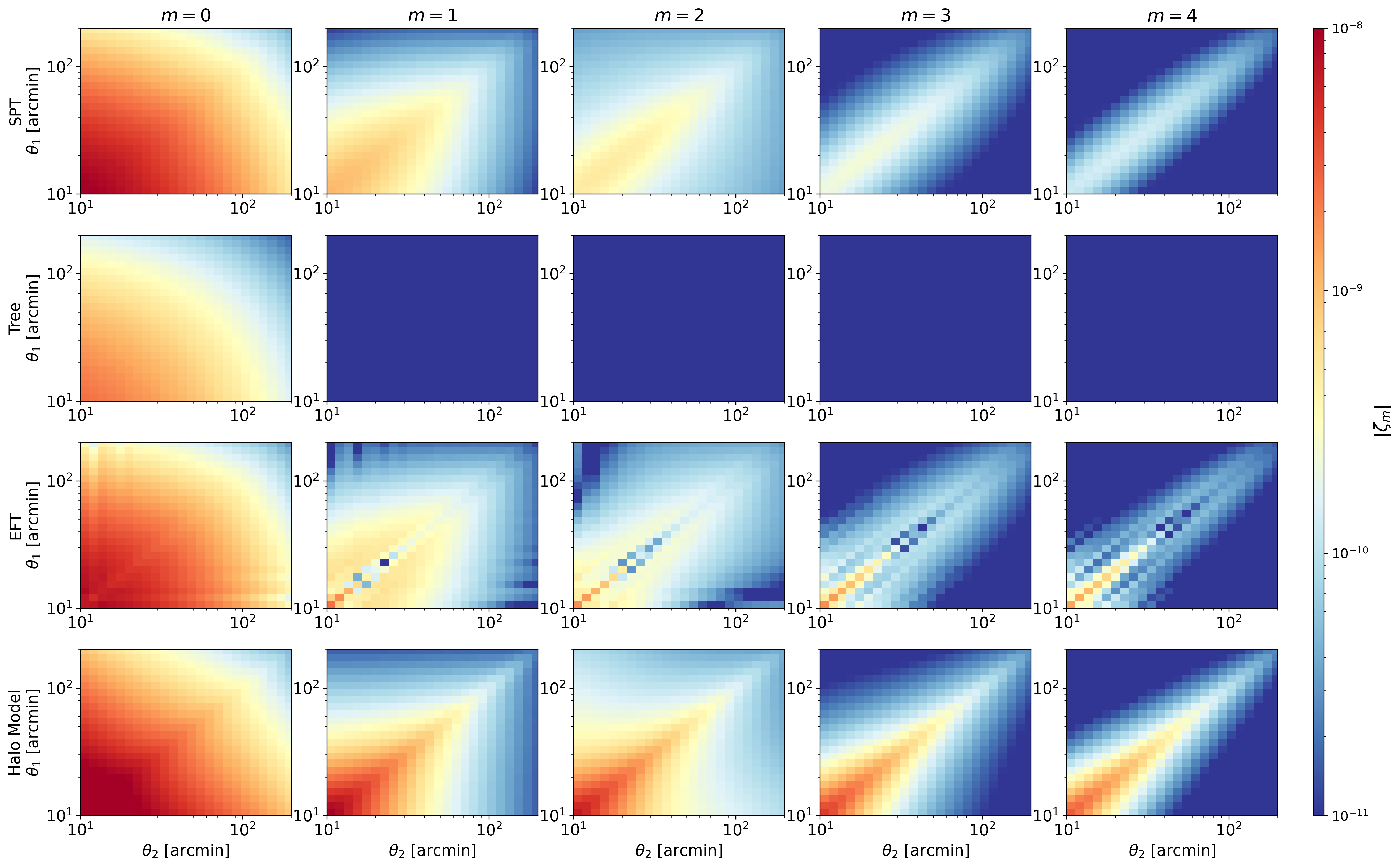
Comparing different models
We can run several theoretical models by changing
tree_level:
base_params = dict(
    numberThreads=8,
    verbose=2,
    verbose_log=1,

    # T17 / paper cosmology
    z=0.5078,
    h=0.7,
    sigma8=0.82,
    Omb=0.046,
    Omc=0.233,
    Omnu=0.0,
    ns=0.97,
    w=-1.0,

    # Make sure this P(k) was generated with the same cosmology
    fnamePS="./input/linear_pk_camb_T17_z05078.txt",

    # Redshift bin
    Wg=0,
    fWgchi="./input/Wg_Takahashi_z05078.txt",

    rootDir="Output",

    zbin=0.5078,
    mMax=5,
    chiQuadSteps=300,
    GLpoints=64,
    Nell=128,
    ellmax=10000,
    ellmin=0.001,
    writevectors=0,
    options=""
)

models = {
    1: ("SPT", "spt"),
    2: ("Tree", "tree"),
    3: ("EFT", "eft"),
    4: ("Halo Model", "halo_model"),
}

for tree_level, (model_name, prefix_name) in models.items():

    print(f"Running {model_name} model with tree_level={tree_level}")

    params = base_params.copy()
    params["tree_level"] = tree_level
    params["prefix"] = f"{prefix_name}_z05078_"

    w = wlcf()
    w.set(params)
    w.Run()

    print(f"Finished {model_name}")
We plot the different cases
plt.rcParams.update({
    "font.size": 14,
    "axes.titlesize": 16,
    "axes.labelsize": 14
})

path = "Output"

models = {
    "SPT": "spt_z05078_",
    "Tree": "tree_z05078_",
    "EFT": "eft_z05078_",
    "Halo Model": "halo_model_z05078_",
}

m_values = range(5)

theta = np.loadtxt(f"{path}/{models['SPT']}theta_array.txt") * 180 / np.pi * 60
Theta2, Theta1 = np.meshgrid(theta, theta)

nrows = len(models)
ncols = len(m_values)

fig = plt.figure(figsize=(20, 13))

gs = fig.add_gridspec(
    nrows=nrows,
    ncols=ncols + 1,
    width_ratios=[1, 1, 1, 1, 1, 0.05],
    wspace=0.2,
    hspace=0.25
)

norm = LogNorm(vmin=1e-11, vmax=1e-8)

for i, (model_name, prefix) in enumerate(models.items()):
    for j, m in enumerate(m_values):

        ax = fig.add_subplot(gs[i, j])

        zeta = np.abs(np.loadtxt(f"{path}/{prefix}zetam{m}.txt"))

        im = ax.pcolormesh(
            Theta2,
            Theta1,
            zeta,
            shading="auto",
            cmap="RdYlBu_r",
            norm=norm
        )

        ax.set_xscale("log")
        ax.set_yscale("log")
        ax.set_xlim(10, 200)
        ax.set_ylim(10, 200)

        if i == 0:
            ax.set_title(fr"$m={m}$")

        if j == 0:
            ax.set_ylabel(f"{model_name}\n" + r"$\theta_1$ [arcmin]")

        if i == nrows - 1:
            ax.set_xlabel(r"$\theta_2$ [arcmin]")

cax = fig.add_subplot(gs[:, -1])
cbar = fig.colorbar(im, cax=cax)
cbar.set_label(r"$|\zeta_m|$", fontsize=16)
cbar.ax.tick_params(labelsize=12)
plt.savefig("models_3pcf.png", dpi=300, bbox_inches="tight")
plt.show()
The Google Colab: Four-Model Comparison notebook packages this comparison into a standalone, directly executable workflow and also adds one-dimensional model slices.
Emulator and MCMC notebooks
The repository also includes a compact emulator workflow under tests/.
The emulator is trained from 3ptWL-mod outputs, so users can regenerate the full
data set instead of relying on precomputed development files.
Run the notebooks in this order:
tests/emulator.ipynbbuilds a 300-point Latin-hypercube grid in
Omega_m,h, andlogAs;generates CAMB linear power spectra;
runs 3ptWL-mod for the zs9 redshift configuration;
trains one neural-network emulator per multipole and saves the weights under
tests/emulator_outputs/.
tests/use_wlcf_emulator.ipynbloads the weights generated by the first notebook;
shows how to evaluate the emulator;
selects a random test-set cosmology;
builds a simple artificial covariance;
runs a short
emceefit and saves a triangular plot undertests/emulator_usage_demo/.
tests/firecrown_emulator_likelihood.ipynbloads the same emulator weights;
builds a masked 3ptWL-mod data vector with the new binning mask;
constructs a Gaussian likelihood with an artificial covariance;
runs a compact
emceecheck;includes an optional Firecrown
StatisticandConstGaussianscaffold that can be activated after installing Firecrown.
The implementation shared by these notebooks lives in
tests/emulator.py. Edit EmulatorConfig in that file, or override it
inside the notebook, to change the parameter ranges, number of evaluations,
network architecture, number of MCMC walkers, or number of MCMC steps.
The Firecrown bridge is optional. If it is needed, install Firecrown and SACC
from conda-forge in the notebook environment:
conda create -n 3ptwl-mod-firecrown -c conda-forge \
  python=3.11 camb scipy scikit-learn matplotlib emcee corner \
  firecrown sacc jupyterlab ipykernel
conda activate 3ptwl-mod-firecrown
python -m ipykernel install --user --name 3ptwl-mod-firecrown \
  --display-name "Python (3ptWL-mod Firecrown)"