Google Colab: Four-Model Comparison

The standalone Colab notebook is the fastest way to run the four public 3ptWL-mod theory branches without cloning the repository. It installs the 3ptWL-mod source distribution from PyPI, downloads one versioned example power spectrum, runs every branch with a common numerical configuration, and plots the results on shared scales.

The notebook source is also available on GitHub.

Models

The labels used in the notebook match the model reference and the tree_level run-time parameter:

Four model branches

Notebook label	tree_level	Physical approximation
SPT	1	Standard perturbation theory.
Tree	2	Power-spectrum-squared approximation.
EFT	3	Effective-field-theory inspired branch.
Halo Model	4	Takahashi/Halo-model inspired branch.

See 3PCF Model Reference for the scientific conventions behind these branches. They are different physical approximations, not successive numerical accuracy levels.

What the Notebook Does

The notebook is independent of a repository checkout. In order, it:

1. installs the native GSL and FFTW3 dependencies available in Colab;

2. installs 3ptWL-mod==1.0.0 from PyPI;

3. downloads linear_pk_Takahashi_z0.txt from the matching v1.0.0 tag;

4. runs SPT, Tree, EFT, and Halo Model with the same input and grid settings;

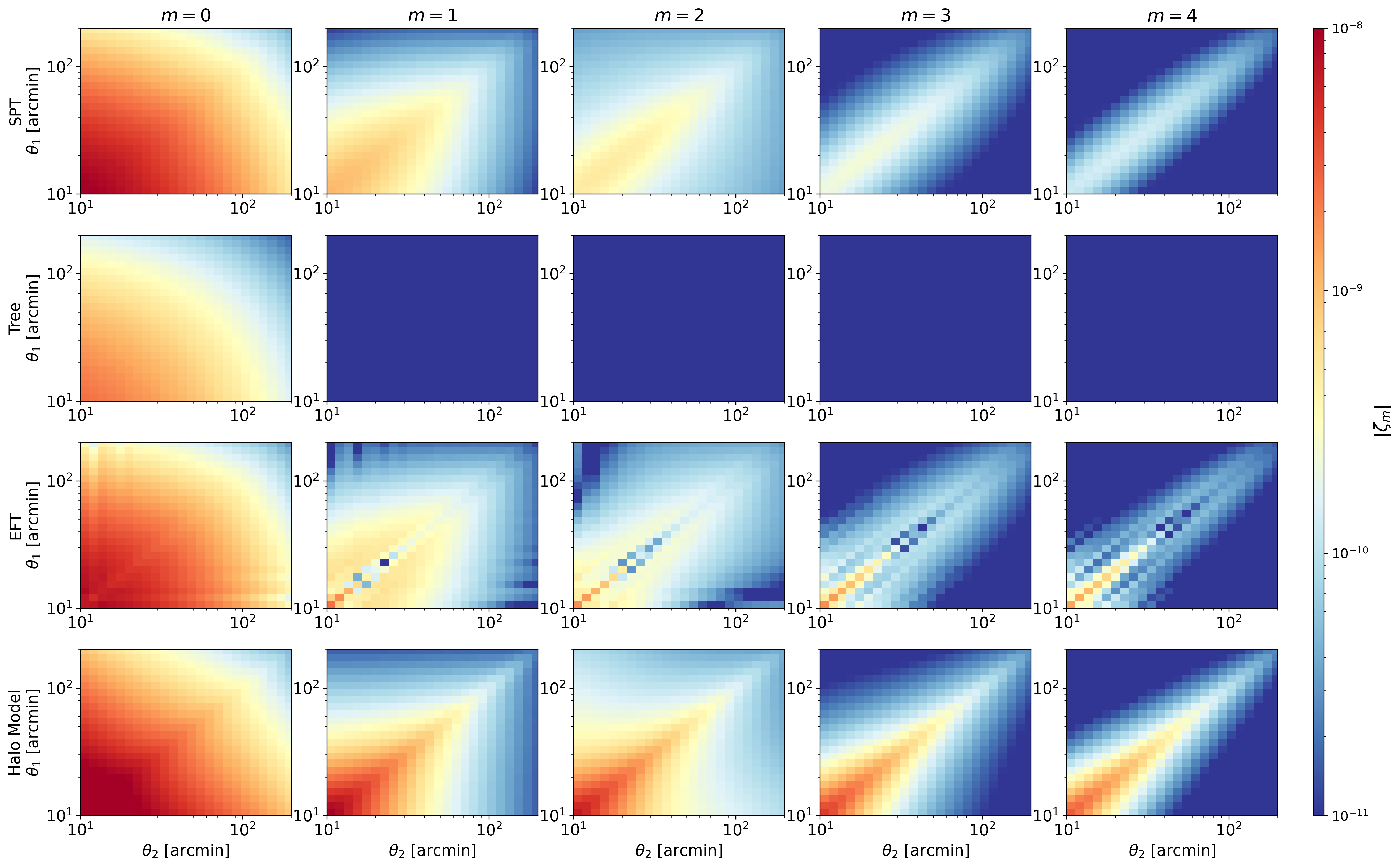
5. creates a four-by-five map of \(|\zeta_m|\) for m=0,...,4;

6. compares one-dimensional slices at three fixed values of \(\theta_2\); and

7. packages the numerical outputs and figures into a zip archive.

The main map uses one logarithmic color scale for all 20 panels. This makes amplitude differences physically visible; a branch whose values fall below the displayed lower bound will therefore appear at the lowest color.

Fast and Higher-Resolution Modes

The default FAST_MODE=True configuration uses:

Nell = 48
chiQuadSteps = 80
GLpoints = 24
mMax = 4

Set FAST_MODE=False to use the repository example settings:

Nell = 64
chiQuadSteps = 120
GLpoints = 32
mMax = 4

Both configurations are tutorial settings. Before using predictions in an analysis, increase the relevant grid controls and establish convergence over the angular range and model branch of interest. Replace the example power spectrum with one generated for the intended cosmology and redshift.

Generated Files

The notebook writes its products beneath 3ptwl_colab/ in the Colab runtime. The principal figures are:

• four_models_3pcf_maps.png;

• four_models_3pcf_slices.png.

The optional final cell creates 3ptwl_four_models_results.zip for download. The runtime filesystem is temporary, so download results before closing the session.

Local Use

The same notebook can be opened locally from examples/3ptWL_mod_four_models_colab.ipynb. Install the native prerequisites described in Installation first. Outside Colab the notebook skips the apt-get step and uses pip in the active Python environment.